Features and Usages

Spreadsheet User Interface Overview

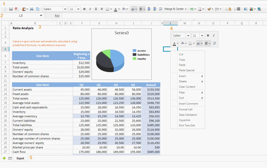
Above is a screenshot of ZK Spreadsheet's user interface, each section is introduced in the following:

1. Toolbar

   The toolbar contains all commonly-used functions including setting cell's style, alignment, border, background color, font, font color, merging (and unmerging) of cells, sorting, auto filter, protection and grid line visibility. It has 2 tabs, another tab is used to insert charts, images, and hyperlinks for web page and email address:

   The 3 leftmost buttons, "New Book", "Save Book", and "Export to PDF", are not built-in functions. You have to implement them by yourself.

2. Formula bar

   It displays editing text or formula of current selected cell and can be used to enter or edit a formula or data.

3. Sheet Area

   It displays the content of current selected sheet, and you usually perform most editing operations in this area.

4. Context menu

   Right clicking on a cell, a column header, or a row header pops up a context menu. It contains most options of the toolbar and works like a shortcut.

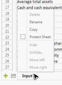
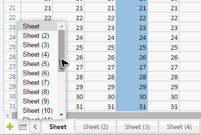
5. Sheet bar

   A list of all sheets in this book. You can navigate to any sheet by clicking on it. Click can add a new sheet. Right clicking on a sheet pops a context menu, and it allows you to do some sheet operations.

   

   Sheet navigation button makes you switch sheets conveniently.

Features

Integrating with ZK Charts

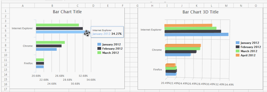
Every chart is now rendered by another ZK product ZK Charts which is more elegant and displayed with animation. When you hover your mouse pointer, it will show related data in a tooltip.

Rich Text Editing

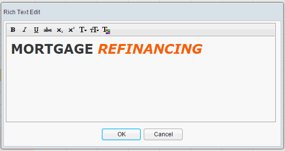
You can apply multiple styles to a cell with a rich text editor. To open a rich-text editor, right clicking a cell, select "Right Text Edit" in the context menu.

Comment

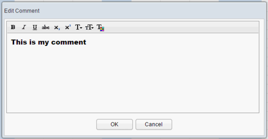
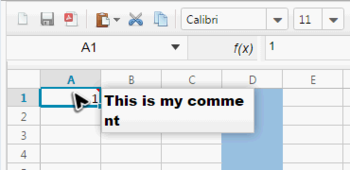
To insert/edit/delete a comment, right clicking a cell, select corresponding item in the context menu.

Support Different Zoom Level

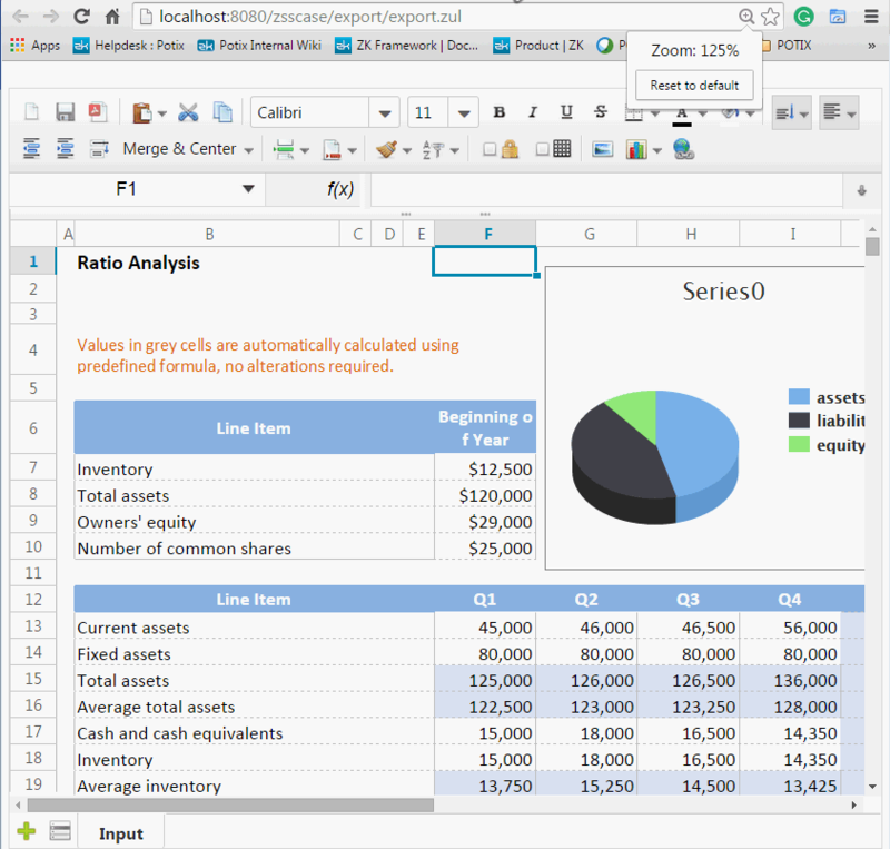
Spreadsheet supports viewing in different zoom level. You can change zoom level within a browser according to your need.

The screenshot below is a Spreadsheet which is zoomed to 150%.

Display Currency Symbol of Different Countries

ZSS can display currency symbol of different countries such as $, ¥, ₩, €, and HKD on a cell with currency format.

Localization of Number/Formula Input

ZSS also accepts ','(comma) or '.'(dot) as the decimal point for decimal numbers.

Smart Input

When you enter a text in a cell with the default format (General), ZSS convert some special number inputs such as 1,234,567, $123456, ($123456), ($1,234,567), 1.2%, 123456E10 into a number value and set its corresponding Cell format automatically.

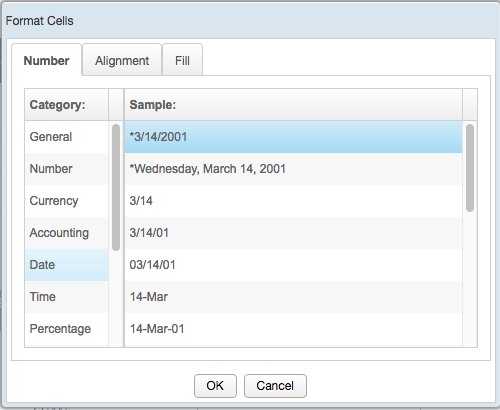
Date Format

Some date formats in ZSS are regional (starting with an asterisk, *, same as Excel ) and some are international.

Regional ones will change its displaying format according to the system locale, but international one doesn't change.

Conditional Formatting

since 3.9.0

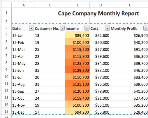
ZSS can display conditional formatting of an Excel file. This feature allows you to highlight a cell with a certain color according to the cell's value like the "Income" column below:

• Modify conditional formatting is not supported yet.

Name Range

ZSS cac read a named range in an xlsx file, so you can specify a named range in a formula e.g. =SUM(source). To create a name range, please call Range::createName.

Supported Hotkeys

Hotkey	Action
CTRL+B	bold
CTRL+C	copy
CTRL+I	italic
CTRL+U	underline
CTRL+V	paste
CTRL+X	cut
CTRL+Y (EE only)	redo
CTRL+Z (EE only)	undo
Delete	clear content
Esc	clear copy/cut clipboard
CTRL+ARROW KEY	moves the selection box to the edge of the current data region in a sheet.

Usage

The following sections will introduce usages of some noticeable features which are all Available in ZK Spreadsheet EE only.

Copy & Paste

We recommend you to copy and paste with Ctrl+c and Ctrl+v which works in all cases rather than clicking "paste" button on the toolbar and "paste" item on the context menu.

Copy inside One Spreadsheet

• Such copy-paste works with Ctrl+c and Ctrl+v, toolbar, and context menu.
• ZSS has full information of cells at both server and client-side, so such paste can retain all information of cells including styles, a formula, format, and data validation.
• If you copy a whole column/row, ZSS also copy the width/height. But copying one or multiple cells doesn't copy the width and height to target cells.
• When copy highlight is still active, it copies the highlighted cells, not from the system clipboard. You need to cancel the copy highlight first, then you can paste from a system clipboard.

Between 2 ZSS components

• Copy-paste cells between 2 ZSS components also rely on the system clipboard, so it's a similar case like ZSS and Excel, only copying pure text.
• If you want to copy a whole sheet to another ZSS component, please call Range.cloneSheetFrom(). It can clone a sheet from another Book object.

Between ZSS and Other Applications like Excel

• Such copy-paste only works with Ctrl+c and Ctrl+v. Click "Paste" on the toolbar or context menu only works for copying cells inside one ZSS component.
• Such copy-paste is an action between 2 applications (e.g. Excel and a browser) through a system clipboard. Currently, ZSS only extract text content from a system clipboard, so this copy-paste only pastes the "pure text" you see on the screen without any specified style on cells.
• For example, a cell in Excel with a formula =sum(1), if you copy the cell and paste it to ZSS, the cell in ZSS gets 1 as a number. Just like you type 1 in a ZSS cell.
• If you enter edit mode, select the text =sum(1) and copy it in Excel, then paste to a cell in ZSS. ZSS gets a formula, just like you type a formula in a ZSS cell.

limitation

ZSS can't paste a cell that has a multiline text into one cell of ZSS, and it will split the text into multiple cells by rows.

Special Paste

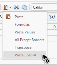
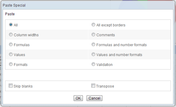
In addition to normal pasting, Spreadsheet also provides other special pasting options on the toolbar.

You can select "Paste Special" to access all available pasting options in a dialog.

Custom Sort

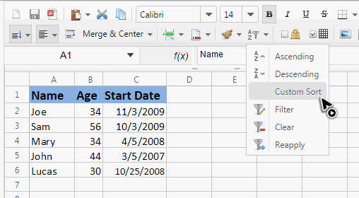
The "Ascending" and "Descending" function can sort data by only one column but "Custom sort" can sort data by multiple columns.

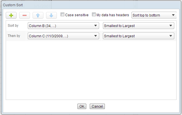
After selecting "Custom sort" on the toolbar, a dialog appears. You can add sorting criteria to 3 columns at the most. If your data includes column headings, make sure the "My data has headers" option is checked.

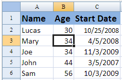
The sorting result of criteria above:

Auto Fill

Auto fill is a handy feature to fill cells with data in a particular pattern based on selected cells. Text will be copied and numbers and dates will be increased (or decreased).

To use this, You should select one or more cells and drag the fill handle across or down the cells that you want to fill.

Fill cells by dragging right, left, up, or down.

The supported cell content are number, weekday (full/short), month (full/short), and timestamp.

Format Cell

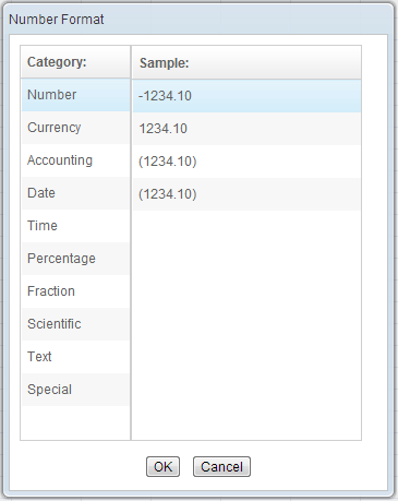
A context menu appears when right clicking a cell, "Format Cell" provides 10 different categories with total of 47 formats to apply on cells.

Sheet Protection

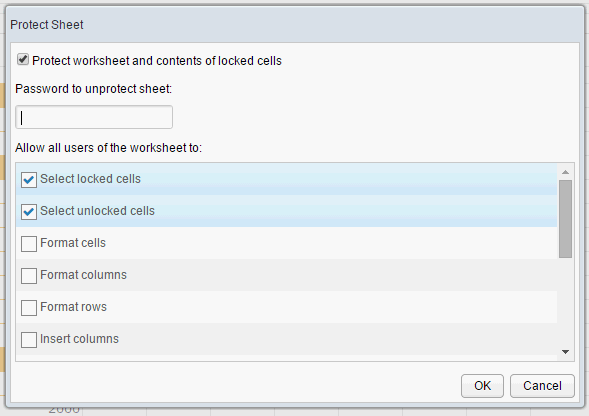
If you enable "Protect Sheet" for a sheet in Excel, Spreadsheet will keep this setting when reading the Excel file, hence, when you edit a protected sheet, you will receive an alert message on the top left-hand corner.

When a sheet is under protection, you can only edit those unlocked cells. For those locked cells, you still can specify which action you allow users to do.

Filters

The filter can help you screen out data and work with a subset of data in a range of cells without moving or deleting them.

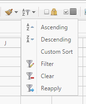
When you click on the filter icon, there are 3 menu items: Filter, Clear, and Reapply related to filter.

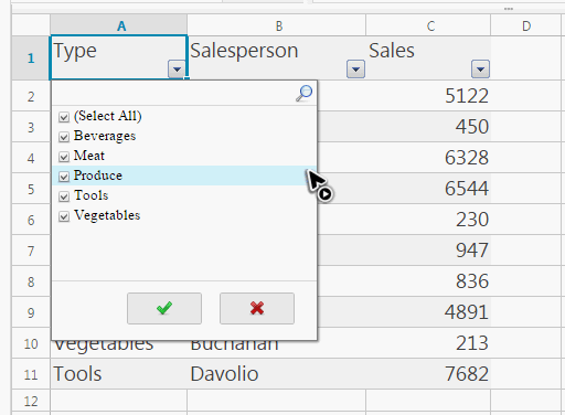
Click "Filter" can enable / disable filters. When filters are enabled, first row of each column will show up a drop-down arrow icon . If you click the drop-down icon, a list of values appears and you can select from the list as a filtering criterion to apply on data.

After you select some values click , Spreadsheet will filter those data with selected values. Only those rows with matching criteria will be displayed while others stay hidden.

You can also filter by multiple columns. Filters are additive, which means that each filter is based on the existing filters and further reduces the subset of data.

Click "Clear" removes all applied criteria and display all data available.

If you add new data row, you should click "Reapply" . Then, drop-down list will update its values, and applied criteria will also work on new data.

since 3.8.1

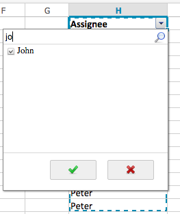
Filter by search. When you enter text in the search box, it will instantly list and select all matched values. Press "Enter" and ZSS will filter your data with those matched values.

since 3.9.0

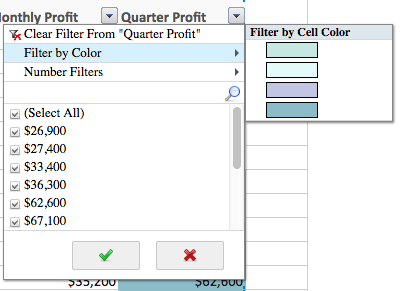
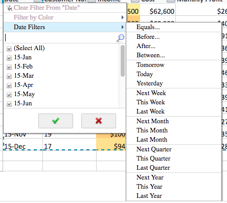
ZSS supports number filter, color filter, date filter, and text filter.

Data Validation

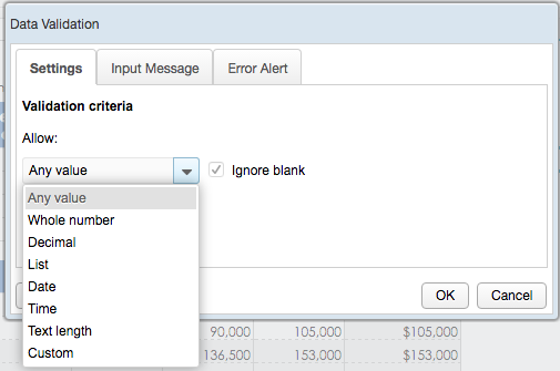
Spreadsheet can read data validation settings of Excel files including validation criteria of lists, numbers, decimals, dates, or time. (Spreadsheet OSE will ignore validation settings.)

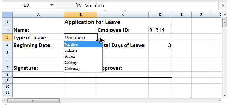
If the validation criteria is a list, the cell will appear a drop-down arrow icon. You can click the icon to select available values.

When you click on the cell with validation, the input message you set will appear automatically.

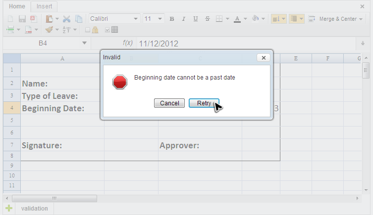
If your input violates validation criteria, an error alert will pop up.

There are 3 types of alerts and each of them has a different icon in the dialog. For an error alert , you can retry to enter again or cancel to revert back to the original value. For a warning alert , you can click "Yes" to accept the invalid input, "No" to edit the invalid input, or "Cancel" to remove the invalid input. For a information alert , you can click "OK" to accept the invalid value or "Cancel" to reject it.

• custom validation is not supported yet.

All source code listed in this book is at Github.